
Allen McNamara on the Deep Mantle Structure of the Earth

Allen McNamara is a Professor of Geological Sciences at Michigan State University. He explains how his computer-based fluid-dynamical models of the mantle help distinguish between competing theories about the nature and origin of the large low-shear-velocity provinces near the core-mantle boundary under Africa and the Pacific.
Listen to the podcast here or wherever you listen to podcasts.
Scroll down for illustrations that support the podcast. And add your comments at the bottom of the page.
Note - playing the podcast is not supported on Internet Explorer; please use any other browser, or listen on Spotify, Apple Podcasts, etc.
Podcast Illustrations
Source citations are listed at the bottom of this page.
Large Low-Shear-Velocity Provinces

Animation showing the extent of the large low-shear-velocity provinces (red) inferred from seismic tomography. The dark red ball represents the Earth’s core.
Courtesy of Sane Cottar

3D rendering of seismic tomography of the lower mantle: low-shear-velocity regions are shown as red and high-shear-velocity regions are shown as blue. The large red regions lying below Africa and the Pacific are the large low-shear-velocity provinces.
Ritsema et al., 2004

Map of the large low-shear-velocity provinces (red) for a layer 200 kilometers above the core-mantle boundary.
Ritsema et al., 2004
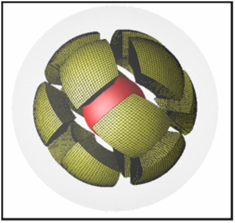
Example of a mesh used in the computer-based fluid dynamical models created by Allen McNamara and his colleagues. The red ball in the center represents the core. The mantle is divided into 12 caps, each of which is handled by a different processor. The mesh extends from the core-mantle boundary at the bottom to the overriding lithosphere at the top (not shown). As computer performance increases, it becomes practicable to use ever-finer meshes. In 2021, 144 processors work in parallel using mesh elements representing a radial increment of 25-50 kilometers.
Modeling of a compositionally distinct primordial layer of mantle around the core

Prediction of the present-day shape of a primordial compositionally differentiated dense layer (orange) at the bottom of the mantle that has been perturbed from an initially smooth layer by the flows induced by plate tectonics acting over the past 120 million years. In the podcast, compositionally differentiated regions are called compositional reservoirs. The image also shows the observed seismic tomography, with blue and red representing faster seismic velocity (i.e., cooler) and slower seismic velocity (i.e., warmer) regions respectively. The following set of images show the seismic tomography predicted by the model.
Hernlund & McNamara, 2015
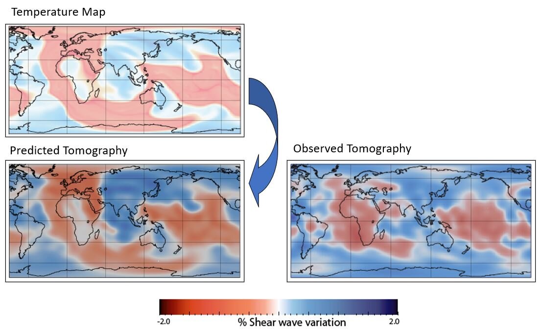
The top left image shows the temperature field that would result from the computer-generated compositional reservoir shown above. If seen through the “eyes” of present-day seismic tomography, the results would be as shown at bottom left. This bears considerable resemblance to the observed seismic tomography shown at bottom right. All maps are for a layer about 200 kilometers above the core-mantle boundary.
Bull et al., 2009
Modeling of a primordial layer of compositionally uniform but cooler mantle around the core

This 3D map shows clusters of plumes that result from modeling the effect of plate motions over the past 120 million years on a primordial, initially uniform layer of cooler mantle without any compositional differentiation from the rest of the mantle.

The top left image shows the temperature field that would result from the plume cluster prediction shown above, with its corresponding hypothetical seismic tomography (bottom left). This bears much less resemblance to the observed seismic tomography (bottom right) than the first example shown above. Thus, according to these models, if the large low-shear-velocity provinces are primordial, an initial smooth layer would have been chemically differentiated as well as cooler, not just cooler. All maps are for a layer about 200 kilometers above the core-mantle boundary.
Bull et al., 2009

There are two main hypotheses as to how compositional reservoirs at the base of the mantle formed: (i) a primordial, intrinsically denser layer continually erodes as it gets caught up in mantle flows (top); and (ii) an intrinsically denser material, such as basalt, subducts and accumulates through time (bottom). Each of these can produce the same present-day result, which makes it hard to determine which is more likely to have occurred. The series of models shown next simulate subduction of various thicknesses of crust to see if the second, i.e., the accumulation hypothesis, is plausible.
Garnero et al., 2016
When subduction of a thin 6-kilometer-thick crust is modeled, no compositional reservoir accumulates at the bottom of the mantle at the core-mantle boundary.
All three simulations from Li et al., in review
When subduction of 30-kilometer-thick crust is modeled, a compositional reservoir accumulates at the bottom of the mantle at the boundary with the core.
In this model, the subducting crust starts off at a thickness of 30 kilometers and becomes thinner with time, ending with a thickness of 6 kilometers. This reflects the idea that when the Earth was younger, a hotter mantle created more melt at spreading ridges, generating a thicker ocean crust. The model suggests that a compositional reservoir is formed but that it has very irregular boundaries.
Model of a primordial reservoir of material that is more primitive and denser (cyan) than the background mantle (black). Cooler material in downwellings (yellow) that arise from the mantle convection are analogous to subducted ocean crust. Oceanic crust that subducted into the mantle has three possible pathways: being stirred into the background mantle; being entrained into mantle plumes; or being flushed into primordial reservoirs.
Li et el., 2014
Ultra-Low-Velocity Zones

Map of ultra-low-velocity zone detections and non-detections. The background shaded regions show the shear-wave tomography of the lowermost mantle. Most of the mantle has not yet been mapped with respect to ultra-low-velocity zones.
McNamara et al., 2010
The model starts off with a thin layer of material even denser than the material forming the large low-shear-velocity provinces. In the animation, the ultra-low-velocity zones are shown in dark red, the large low-shear-velocity provinces are shown in red, the background mantle appears black, and the light-colored wisps are subducted crust. The model shows how the ultra-low-velocity material eventually accumulates at the edge of the large compositional reservoirs, rather like dirt accumulating at the bottom of a pool where eddies converge.
McNamara et al., 2010
Zooming in to the ultra-low-velocity zone simulation. The simulation shows that when the ultra-low-velocity zones (dark red) occur on the edges of the compositional reservoirs, they develop asymmetrical shapes, with a steeper profile on the outer edge of the reservoir where the temperature is lower and they become more viscous.
McNamara et al., 2010
References
Bull, A.L., A.K. McNamara, and J. Ritsema, Synthetic tomography of plume clusters and thermochemical piles, Earth and Planetary Science Letters, 278, 152-162, 2009.
Garnero, E.J., A.K. McNamara, and S.-H. Shim, Continent-sized anomalous zones with low seismic velocity at the base of the Earth's mantle, Nature Geoscience, 9, 481-489, doi:10.1038/NGEO2733, 2016.
Hernlund, J.W., and A.K. McNamara, The Core-Mantle Boundary Region, in Gerald Schubert (editor-in-chief) Treatise on Geophysics, 2nd edition, Volume 7. Oxford: Elsevier; 2015. p461-519
Li, M., A.K. McNamara, and E.J. Garnero, Chemical complexity of hotspots caused by cycling oceanic crust through mantle reservoirs, Nature Geoscience, 7, 336-370, doi:10.1038/ngeo2120, 2014.
Li, M., and A.K. McNamara, The evolving storage of subducted oceanic crust in Earth’s lowermost mantle, Earth and Planetary Science Letters, in review.
McNamara, A.K., E.J. Garnero, and S. Rost, Tracking deep mantle reservoirs with ultra-low-velocity zones, Earth and Planetary Science Letters, 299, 1-9, 2010.
Ritsema, J., van Heijst, H.J., Woodhouse, J.H., Global transition zone tomography, Journal of Geophysical Research, B 109, 2004