
Carolina Lithgow-Bertelloni on Dynamic Topography

Carolina Lithgow-Bertelloni is a Professor of Geosciences at the University of California, Los Angeles. She views the Earth’s large-scale topography as an expression of the interior processes of the Earth, and in particular of the currents in the mantle. She describes how this works, and gives examples of major topographic features that are best explained by invoking vertical motions of the mantle.
Courtesy of Carolina Lithgow-Bertelloni
Listen to the podcast here or wherever you listen to podcasts.
Scroll down for illustrations that support the podcast.
Note - playing the podcast is not supported on Internet Explorer; please use any other browser, or listen on Spotify, Apple Podcasts, etc.
Podcast Illustrations
All illustrations courtesy of Carolina Lithgow-Bertelloni unless otherwise noted.

Diagram illustrating the principle of dynamic topography. Differences in density in the mantle induce the flow indicated by the arrows. This flow exerts forces on the base of the overriding tectonic plates, causing a deflection in the surface.

Cartoon showing the two main contributions to topography: isostatic, which is a result of variations in thickness and density of the crust and lithospheric mantle; and dynamic, which is caused by deflection of the Earth’s surface by vertical forces imposed on it by mantle convection. The two inset columns illustrate isostatic topography, and dynamic topography is shown above a subduction zone (left, blue arrows) and an upwelling under a continent (right, yellow arrows).

Maps of the large low-shear-velocity provinces detected by seismic tomography. The top figure shows a 3D rendering of the boundary of the provinces. The lower figure is a map of a slice through the lowermost mantle at a depth of 2750 km. They show that the low-velocity regions lie primarily below Africa and the Pacific. The low-velocity regions are interpreted as higher temperature regions that are expected to generate upward convective flow patterns.
Courtesy of Allen McNamara, based on the S20RTS tomography model by Ritsema et al., 1999, 2004

Map of the residual global topography after the isostatic component caused by the thickness and density of the lithosphere is subtracted from the present-day observed topography. The major cause of this topography is thought to be the dynamic topography discussed in the podcast. Prominent high regions (red) are seen under the Western Pacific, the Eastern Africa, Antarctica, and the North Atlantic.

Reconstruction of the effect of subduction of the Farallon plate off the west coast of North America about 60 million years ago. The shaded region labeled dynamic subsidence would have been sufficiently depressed to allow incursion of the shallow inland seas for which there is ample evidence in the fossil record.
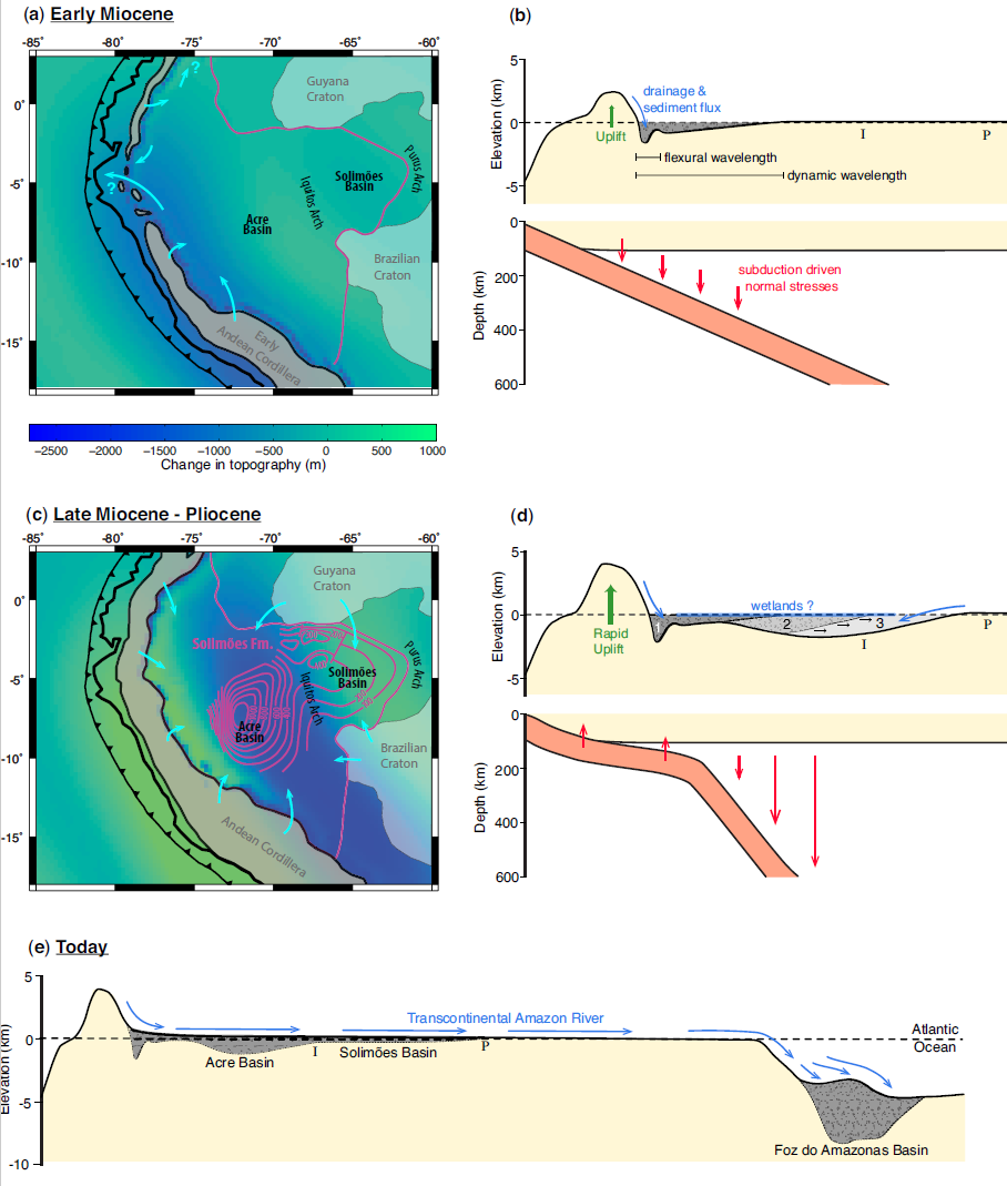
Schematic illustrations showing how a change in subduction style could have driven the topographic and sedimentary evolution of western Amazonia in South America since the Miocene (23 million years ago), eventually shaping the present day landscape. Figures (a) and (c) map the topography predicted by flexural and dynamic calculations both before and after the arrival of the flat slab. Turquoise arrows represent drainage directions. Gray dotted regions indicate sedimentary infill, with region 1 being the oldest deposits and 3 the youngest. Figure (e) is a similar cross-section extending from the offshore trench to the Atlantic Ocean, showing the present day configuration of drainage and the location of the sedimentary deposits that preserve the record of landscape evolution hypothesized in figures (b) and (d).
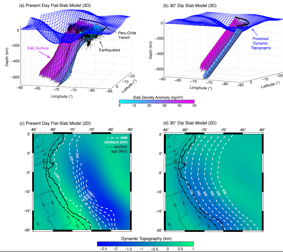
Comparison of dynamic topography predicted by two different slab models for the Peruvian subduction zone, shown in 3D (top row) and 2D (bottom row). The left-hand side (a and c) represents the present-day 3D flat-slab morphology determined from local seismicity (small black circles give individual earthquake locations), whilst the right-hand side (b and d) reflects the uniform 30◦ dip slab model akin to ‘normal’ subduction before the onset of slab flattening.
(a–b) Dynamic topography (blue mesh surfaces) has been vertically exaggerated for illustrative purposes. The slab surfaces are color-coded according to the density assigned in the models. (c–d) Same as figures (a–b) but now in map view, comparing the dynamic topography with the slab contours (white dashed lines).