
Patrick Fulton on the 2011 Tōhoku Earthquake
Listen to the podcast here, or wherever you get your podcasts.

Patrick Fulton uses observation, quantitative analysis, and numerical modeling to study heat and fluid in fault zones. He applies his research to the physics of earthquakes, tectonic processes, and the transport of subsurface heat and fluids. In the podcast, he describes how he and his team installed a borehole “temperature observatory” below 7 km of ocean. The observatory detected the remnants of frictional heating generated by the slip that caused the 2011 Tōhoku Earthquake and the devastating tsunami that led to the Fukushima nuclear disaster.
Patrick Fulton is an Assistant Professor in the Department of Earth and Atmospheric Sciences at Cornell University.
Podcast Illustrations
Images courtesy of Patrick Fulton unless otherwise indicated.
Drill Site Setting

Google Earth image of Japan and a portion of the western Pacific. The Pacific plate is subducting at the Japan trench, which is the dark feature extending from top right to the bottom of the image. The earthquake epicenter was about 45 miles off the eastern coast of Honshu, Japan’s largest island.

Map of the 2011 Tōhoku earthquake region, with the red star showing the earthquake’s epicenter. The Japanese island of Honshu sits on the small Okhotsk plate. The Pacific plate is subducting under the Okhotsk plate at the Japan trench, and is moving to the west northwest towards the trench, as indicated by the large black arrow. The shaded regions bounded by the solid contours indicate the amount of seafloor movement during the earthquake. The site of the borehole observatory discussed in the podcast is shown by the red dot labeled JFAST Site C0019. The other red dots show other sites where core samples were drilled and used for comparison with those from the JFAST borehole. The dotted line shows the extent of seafloor slip accompanying a tsunami-generating earthquake that occurred in 1896.
Chester, F.M. et al. (2013), Science 342, 1208

Seismic profile through the borehole site. The profile is annotated to show the accretionary prism (grey), ocean sediments (yellow), and oceanic igneous crust (green). The inferred location of the boundary fault between the Pacific Plate and faults in the overlying sediments is marked as black lines. The location of the borehole (C0019) discussed in the podcast is shown in red, and the black lines at right show locations of other boreholes.
Chester, F.M. et al. (2013), Science 342, 1208

Detail of the region marked by the rectangle shown in the seismic profile shown above. The pattern of lines indicates the various surfaces from which seismic reflections were received. The most significant feature is a faint but continuous reflecting boundary, which is interpreted as the plate-boundary fault.

A main goal of the JFAST project was to measure the increase in temperature at the fault rupture and use that to infer the shear stress. The weight of the overlying rocks provides an estimate of the normal stress. Plugging these numbers into the formula gives the coefficient of friction along the slip surfaces.

The Chikyu deep-sea drilling vessel used to drill the JFAST borehole operated near its limit to install a borehole below nearly 7 km of ocean.
JAMSTEC/IODP
Installing the Temperature Observatory

The JFAST borehole was located on the seafloor below 6,925 m of ocean. The hole extended 850 m into the sub-seafloor rocks, crossing the plate-boundary fault at about 818 m below the seafloor (mbsf). The JFAST team inserted a string of 55 temperature-sensing data loggers attached to a rope installed within a 4.5-inch steel casing. The spacing of the sensors varied, as shown in the figure, so as to maximize the spatial resolution in the temperature-profile measurement near the fault, while still obtaining sufficient measurements along the full length of the borehole to determine steady heat flow and the thermal effects of fluid flows.
Fulton, P.M. et al. (2013), Science 342, 1214

The 55 temperature-sensing data loggers were encased in titanium to withstand the intense pressure. The loggers were then attached to a 830-m-long string with the varying spacing indicated above before insertion into the 4.5-inch steel casing shown below.

Lengths of the 8.5-in drill pipe stacked up aboard the Chikyu. The sensor string with wrapped temperature sensors is strung up in front.
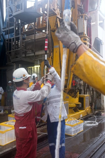
Wrapping protective tape around the temperature sensors before inserting the sensor string into the steel casing.

The assembled temperature observatory (4.5-in steel casing and sensor string) was lowered into the drilled borehole on the seafloor at the end of the drill pipe. The yellow-flanged connector (top center) connects the bottom of the drill pipe (off the top of the picture) to the wellhead assembly fixed to the top of the observatory (center), with the observatory’s steel casing disappearing through the deck into the ocean (lower center).
Core Samples from the Borehole

Core samples extracted from the borehole were analyzed to help determine the location of the fault that slipped during the earthquake. In one technique, the cores were passed through a gamma ray detector to determine the level of naturally occurring gamma rays emitted by the rock. Shales usually emit more gamma rays than other sedimentary rocks due to the high radioactive potassium content of the clay they contain, as well as their high uranium and thorium content.
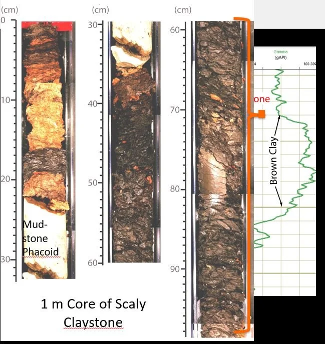
Superposed image at left: a one-meter-long section of the core sample extracted from the borehole at a depth of 820 m below the seafloor at the inferred location of the plate-boundary fault. Right: Profile of the gamma rays emitted by the core sample. The meter-long section in the superposed image at left corresponds to the small orange rectangle on the gamma ray profile. The gamma rays clearly delineate the extent of the brown clay that is thought to mark the plate-boundary surface.

Closeup of an 8.4-cm length of the borehole core at the plate-boundary fault zone. The image shows many small slip surfaces, including one between the red-brown (top) and dark brown (bottom) scaly clays.
Chester, F.M. et al. (2013), Science 342, 1208
Installing the Temperature Observatory

Installation of the observatory below 7 km of ocean required a number of steps. First, a 20-inch casing was installed down to a depth of 27 m below the seafloor, with the top end protruding 3 m above the seafloor. This provided a stable hole at the seafloor to permit further reentries. The drill pipe was then brought up to the ship, and an 8.5-in drill bit was attached to the end of the drill pipe to drill beyond the initial 27 m down to 855 m below the seafloor. The drill pipe was again brought back up to the ship, and the 830 m-long observatory was constructed. This consisted of 4.5-in steel tubing with the sensor string hanging inside it. This assembly was connected to the drill pipe and lowered to the seafloor. The bottom of the assembly was maneuvered so as to enter the borehole. Once fully inserted, the drill pipe was released from the observatory, which was left in place for nine months to record temperature and other data.
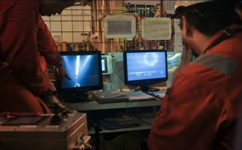
The driller’s “dog house” aboard the Chikyu drill ship. The view from the underwater TV camera shown at right is output on the monitors. In the podcast, Patrick Fulton describes how the long drill pipe behaved like a wet spaghetti noodle. This made it very challenging to maneuver the bottom of the drill pipe and reenter the borehole with the 8.5-in drill bit, and then again with the observatory assembly. When the borehole casing was spotted by the ROV video camera, the captain moved the ship slowly until the hole could be reentered.

After the drilling of the borehole was completed, the video camera shown here was lowered along the drill pipe to provide imagery to guide the crew while attempting to reenter the borehole to insert the observatory assembly.
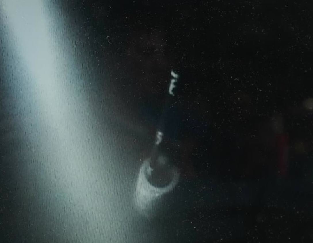
Video frame from the underwater camera shown above as the observatory, i.e., the 4.5-inch steel casing containing the sensor string, was inserted into the borehole.
The steel casing was closed at the bottom but open at the top. Water filled the inside of the casing from the top. The relatively small inner diameter of the casing prevented convection cells from forming. Once inserted, surrounding rocks and sediments collapsed down along the side of the casing, providing good thermal contact with the surroundings. The huge mass of the rock and its enormous thermal capacity overwhelm any influence of heat conduction along the steel casing on the variation of temperature with depth.

The JFAST team aboard the Chikyu deep-sea scientific drilling ship after successful completion of the drilling and emplacement of the temperature observatory.
JAMSTEC/IODP
Retrieving the Sensor String

In April 2013, nine months after installation of the temperature observatory, the team returned in the R/V Karei. From the ship, they operated a deep-sea remotely operated vehicle (ROV) to dive to the seafloor and retrieve the sensor string from the borehole.

The Kaiko II deep-sea ROV was used to locate and retrieve the temperature sensors from the borehole. It was equipped with a video camera and robot arm.

ROV camera image from the seafloor with the ROV robot arm approaching the borehole casing wellhead.
The ROV camera captured this video of its robot arm unlocking the top of the top of the 820-m-long temperature-sensor string to begin pulling it out of the borehole.
JAMSTEC

Hauling the sensor string onto the deck of the R/V Karei.

The full length of the sensor string was laid out on deck following completion of the recovery.
Temperature Observatory Results

Time-space map of the sub-seafloor residual temperature field. The residual temperature is the difference between the measured temperature and the background geotherm, i.e., the steady-state temperature profile of the rocks. The yellow dots at left show sensor positions, and each row represents the corresponding sensor’s data. The blue region at left shows the low temperatures relative to the background geotherm reflecting the effects of water circulation caused by drilling and installation of the sensors. A magnitude 7.3 local earthquake occurred on December 7, 2012 (dashed line), and is thought to have affected the flow of fluids, causing the observed cooling and heating in the high-permeability zones at 784 meters below seafloor (mbsf) and 763 mbsf respectively.

A. Magnified view of of the residual temperature near the plate boundary. B. Simulated residual temperature from a model in which the fault is placed at the peak in the observed temperature anomaly, i.e., 819.8 mbsf. The fault location inferred from the temperature data is at the same stratigraphic level as the plate-boundary fault found in the neighboring coring and logging holes. As discussed in the podcast, these temperature measurements enabled Patrick Fulton and his team to determine a coefficient of dynamic friction on the fault surface of 0.08. This is about an order of magnitude lower than for most rock surfaces, and may help explain the large slip at shallow depths of the fault that contributed to the devastating tsunami.
Fulton, P.M. et al. (2013), Science 342, 1214